Machine Learning Concepts (Part 1)
Content
- Content
- Linear Regression Assumption
- Categorization of ML Algorithms
- Algorithm selection Tips
- How to Prepare for ML-DL Interview
- Difference between Parametric and Non-Parametric model?
- Linear Regression
- Bias Variance Trade-off from Frequentist viewpoint
- Linear Models
- K-means vs kNN
- Nearest Neighbour
- Eigen Decomposition
- Matrix Factorization
- What is NMF?
- PCA and SVD
- Explain PCA? Tell me the mathematical steps to implement PCA?
- Determinant
- Recommendation System:
- Solve Linear Programming
- What is LBFGS algorithm?
- Second-Order Methods: Newton’s Method
- Gradient, Jacobian, Hessian, Laplacian and all that
- Why does L1 regularization induce sparse models?
- Clustering Algorithm
- How to implement regularization in decision tree, random forest?
- Why random column selection helps random forest?
- How to avoid Overfitting?
- How to avoid Underfitting?
- Gaussian Processing
- K-Means Clustering (Unsupervised Learning)
- PCA and Kernel PCA
- Generative Model (Unsupervised Learning)
- Ensemble Method (Bagging and Boosting)
- Online Learning
- Model/ Feature Selection and Model Debugging
- Bayesian Machine Learning
- Finding similar sets from millions or billions data
 Top Pick for Interview - Depth and Breadh
Linear Regression Assumption
There are four assumptions associated with a linear regression model:
- Linearity: The relationship between $X$ and the mean of $Y$ is linear.
-
Homoscedasticity: The variance of
residual($(Y - \hat Y)$) is the same for any value of $X$. - Independence: Observations are independent of each other.
-
 Normality: For any fixed value of $X$, $Y$ is normally distributed. The error($\epsilon = (Y_i - \hat{Y_i})$ residuals) follow a normal distribution $\mathcal{N}(\mu , \sigma)$
Reference:
Categorization of ML Algorithms
To aid our conceptual understsanding, each of the algorithms can be categorized into various categories:
- eager vs lazy
- batch vs online
- parametric vs nonparametric
- discriminative vs generative
![]() Eager vs lazy learners: Eager learners are algorithms that process training data
Eager vs lazy learners: Eager learners are algorithms that process training data immediately whereas lazy learners defer the processing step until the prediction. In fact, lazy learners do not have an explicit training step other than storing the training data. A popular example of a lazy learner is the Nearest Neighbor algorithm.
![]() Batch vs online learning: Batch learning refers to the fact that the model is learned on the
Batch vs online learning: Batch learning refers to the fact that the model is learned on the entire set of training examples. Online learners, in contrast, learn from one training example at the time. It is not uncommon, in practical applications, to learn a model via batch learning and then update it later using online learning.
![]() Parametric vs nonparametric models: Parametric models are
Parametric vs nonparametric models: Parametric models are fixed models, where we assume a certain functional form for $f(x) =y$ . For example, linear regression can be considered as a parametric model with $h(x) = w_1 x_1+ \dots + w_m x_m+b$ . Nonparametric models are more flexible and do not have a pre-specfied number of parameters. In fact,the number of parameters grows typically with the size of the training set. For example, a decision tree would be an example of a nonparametric model, where each decision node(e.g., a binary True/False assertion) can be regarded as a parameter.
![]() Discriminative vs generative: Generative models (classically) describe methods that model the
Discriminative vs generative: Generative models (classically) describe methods that model the joint distribution $P(X,Y) = P(Y)P(X \vert Y) =P(X)P(Y \vert X)$ for training pairs $(x_i,y_i)$. Discriminative models are taking a more direct approach, modeling $P(Y \vert X)$ directly. While generative models provide typically more insights and allow sampling from the joint distribution, discriminative models are typically easier to compute and produce more accurate predictions. Helpful for understanding discriminative models is the following analogy:
Discriminative modeling is like trying to extract information $Y$
given(from) text $X$ in a foreign language ($P(Y \vert X)$) without learning that language.
Reference:
Algorithm selection Tips
- When to use and when not to use.
- Merits and Demerits
- Pros and Cons
How to Prepare for ML-DL Interview
Interviews are stressful, even more so when they are for your dream job. As someone who has been in your shoes, and might again be in your shoes in the future, I just want to tell you that it doesn’t have to be so bad. Each interview is a learning experience. An offer is great, but a rejection isn’t necessarily a bad thing, and is never the end of the world. I was pretty much rejected for every job when I began this process. Now I just get rejected at a less frequent rate. Keep on learning and improving. You’ve got this!
Difference between Parametric and Non-Parametric model?
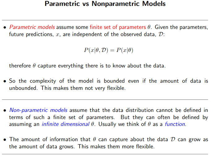
![]() Parametric Model: We have a finite number of parameters. And once you have determined the right parameters, you can throw away the training data. The prediction is based on the learnt weight only.
Parametric Model: We have a finite number of parameters. And once you have determined the right parameters, you can throw away the training data. The prediction is based on the learnt weight only.
… prediction is independent of the training data …
Linear models such:
- Linear regression
- Logistic regression
- Linear Support Vector Machines
- Mixture Models, K-Means
- HMM
- Factor Analysis
These are typical examples of a parametric learners.
![]() Nonparametric Model: The number of parameters is (potentially) infinite. Here number of parameters are function of number of training data.
Nonparametric Model: The number of parameters is (potentially) infinite. Here number of parameters are function of number of training data.
… prediction is dependent of the training data …
Non-parametric models assume that the data distribution cannot be defined in terms of such a finite set of parameters. Model parameters actually grows with the training set. You can imagine each training instance as a “parameter” in the model, because they’re the things you use during prediction
- K-nearest neighbor - all the training data are needed during prediction.
- Decision trees - All the training data needed during prediction. The test input will pass through each decision tree (each decision tree is nothing but some automatic rules based on the full training data) and finally some voting to get the actual prediction.
- RBF kernel SVMs
- Gaussian Process
- Dirichlet Process Mixture
- infinite HMMs
- Infinite Latent Factor Model
These are considered as non-parametric
- In the field of statistics, the term parametric is also associated with a specified probability distribution that you assume your data follows, and this distribution comes with the finite number of parameters (for example, the mean and standard deviation of a normal distribution).
- You don’t make/have these assumptions in non-parametric models. So, in intuitive terms, we can think of a non-parametric model as a
“distribution” or (quasi) assumption-free model.
Reference:
Linear Regression
- It’s linear with respect to weight
w, but not with respect to inputx. posterior ~ likelihood * prior- Ordinary Least Square (OLS) approach to find the model parameters is a
- special case of maximum likelihood estimation
- The overfitting problem is a general property of the MLE. But by adopting the Bayesian approach, the overfitting problem can be avoided.
[p9, Bishop]
- Also from Bayesian perspective we can use model for which number of parameters can exceed the number of training data. In Bayesian learning, the effective number of parameters adapts automatically to the size of the data.
Point Estimate of W vs W Distribution
Consider $D$ is our dataset and $w$ is the parameter set. Now in both Bayesian and frequentist paradigm, the likelihood function $P(D \vert w)$ plays a central role. In frequentist approach, $w$ is considered to be fixed parameter, whose value is determined by some form of estimator and the error bars on the estimator are obtained by considering the distribution of possible data sets $D$.
However, in Bayesian setting we have only one single datasets $D$ (the observed datasets), and the uncertainty in parameters is expressed through a probability distribution over $w$. [p22-p23]
![]() A widely used frequentist estimator is the maximum likelihood, in which $w$ is set to the value that maximizes $P(D \vert w)$. In the ML literature, the
A widely used frequentist estimator is the maximum likelihood, in which $w$ is set to the value that maximizes $P(D \vert w)$. In the ML literature, the negative log of the likelihood is considered as error function. As the negative log is a monotonically decreasing function, so maximizing the likelihood is equivalent to minimizing the error.
However Bayesian approach has a very common criticism, i.e. the inclusion of prior belief. Therefore, people try to use noninformative prior to get rid of the prior dependencies. [p23].
Criticism for MLE
- MLE suffers from
overfittingproblem. In general overfitting means the model fitted to the training data so perfectly that if we slightly change the data and get prediction, test error will be very high. That means the model is sensitive to the variance of data. - The theoretical reason is MLE systematically undermines the variance of the distribution. See proof
[[p27], [figure 1.15,p26, p28]]. Because heresample varianceis measured using thesample mean, instead of the population mean. - Sample mean is an unbiased estimator of the population mean, but sample variance is a biased estimator of the population variance.
[p27], [figure 1.15,p26] - If you see the image
p28, the 3 red curve shows 3 different dataset and the green curve shows the true dataset. And the mean of the 3 red curves coincide with the mean of the green curve, but their variances are different.
In Bayesian curve fitting setting, the sum of squared error function has arisen as a consequence of maximizing the likelihood under the assumption of Gaussian noise distribution.
Regularization allows complex models to be trained on the datasets of limited size without severe overfitting, essentially by limiting the model complexity. [p145, bishop]
In bayesian setting, the prior works as the Regularizer.
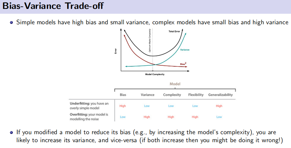
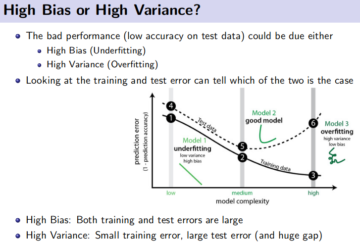
Bias Variance Trade-off from Frequentist viewpoint
The goal to minimize a model’s generalization error gives rise to two desiderata:
- Minimize the training error;
- Minimize the gap between training and test error.
![]() Minimize the training error - Reducing Bias:
This dichotomy is also known as bias-variance trade-off. If the model is not able to obtain a low error on the training set, it is said to have
Minimize the training error - Reducing Bias:
This dichotomy is also known as bias-variance trade-off. If the model is not able to obtain a low error on the training set, it is said to have high bias. This is typically the result of erroneous assumptions in the learning algorithm that cause it to miss relevant relations in the data.
![]() Minimize the gap between training and test error - Reducing Variance:
On the other hand, if the gap between the training error and test error is too large, the model has high variance. It is sensitive to small fluctuations and models random noise in the training data rather than the true underlying distribution.
Minimize the gap between training and test error - Reducing Variance:
On the other hand, if the gap between the training error and test error is too large, the model has high variance. It is sensitive to small fluctuations and models random noise in the training data rather than the true underlying distribution.
In frequentist viewpoint, w is fixed and error bars on the estimators are obtained by considering the distribution over the data $D$. [p22-23; Bishop].
Suppose we have large number of data sets, [D1,...,Dn], each of size N and each drawn independently from distribution of P(t,x). For any given data set Di we can run our learning algorithm and get a prediction function y(x;Di). Different datasets from the ensemble will give different prediction functions and consequently different values of squared loss. The performance of a particular learning algorithm is then assessed by averaging over this ensemble of datasets. [p148; Bishop].
Our original regression function is Y and say for Di we got our predictive function $\hat{Y_i}$.
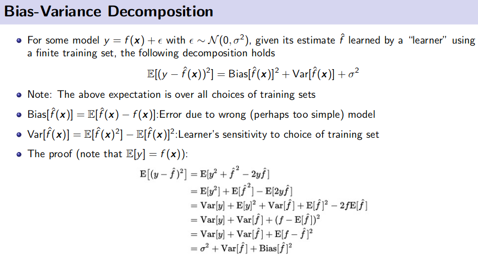
![]() Bias = $(E[\hat{Y_i}(x;D_i)] - Y)^2$, where $E[\hat{Y_i}(x;D_i)]$ is average (expected) performance over all the datasets. So, Bias represents the extent to which the average prediction over all the datasets $D_i$ differ from the desired regression function $Y$.
Bias = $(E[\hat{Y_i}(x;D_i)] - Y)^2$, where $E[\hat{Y_i}(x;D_i)]$ is average (expected) performance over all the datasets. So, Bias represents the extent to which the average prediction over all the datasets $D_i$ differ from the desired regression function $Y$.
-
 TL;DR: The bias of an estimator $\hat \beta$ is the difference between its expected value $E[\hat \beta]$ and the true value of a parameter $\beta$ being estimated: $Bias = E[\hat \beta] − \beta$
![]() Variance = $E[(\hat{Y_i}(x;D_i) - E[\hat{Y_i}(x;D_i)])^2]$, where $(\hat{Y_i}(x;D_i)$ is the predictive function over data set $D_i$ and $E[\hat{Y_i}(x;D_i)])$ is the average performance over all the datasets. So variance represents, the extent to which the individual predictive functions $\hat{Y_i}$ for dataset $D_i$ varies around their average. And thus we measure the extent by which the function $Y(x;D)$ is sensitive to the particular choice of the data sets.
Variance = $E[(\hat{Y_i}(x;D_i) - E[\hat{Y_i}(x;D_i)])^2]$, where $(\hat{Y_i}(x;D_i)$ is the predictive function over data set $D_i$ and $E[\hat{Y_i}(x;D_i)])$ is the average performance over all the datasets. So variance represents, the extent to which the individual predictive functions $\hat{Y_i}$ for dataset $D_i$ varies around their average. And thus we measure the extent by which the function $Y(x;D)$ is sensitive to the particular choice of the data sets. [p149; Bishop]
-
 TL;DR: The variance is simply the statistical variance of the estimator $\hat \beta$ and its expected value $E[\hat \beta]$ , i.e $Var = E [(\hat{\beta} - E[\hat \beta])^2]$
*Note: here patameter $\beta$ and estimator $\hat \beta$.
Bias Variance Decomposition
Resource:
Linear Models
General Linear Model
Indeed, the general linear model can be seen as an extension of linear multiple regression for a single dependent variable. Understanding the multiple regression model is fundamental to understand the general linear model.
Single Regression
One independent variable and one dependent variable
Multiple Regression
Multiple regression is an extension of simple linear regression. It is used when we want to predict the value of a variable based on the value of two or more other variables. The variable we want to predict is called the dependent variable (or sometimes, the outcome, target, response or criterion variable).
![]() TL;DR: Single dependent/target/response variable and multiple ($\gt 1$) predictors/independent variables.
TL;DR: Single dependent/target/response variable and multiple ($\gt 1$) predictors/independent variables.
Multiple linear regression is the most common form of linear regression analysis. As a predictive analysis, the multiple linear regression is used to explain the relationship between one continuous dependent variable and two or more independent variables
Additive Model:
A generalization of the multiple regression model would be to maintain the additive nature of the model, but to replace the simple terms of the linear equation $\theta_i * x_i$ with $\theta_i * f_i(x_i)$ where $f_i()$ is a non-parametric function of the predictor $x_i$.
In other words, instead of a single coefficient for each variable (additive term) in the model, in additive models an unspecified (non-parametric) function is estimated for each predictor, to achieve the best prediction of the dependent variable values.
General Linear Model - Revisited
One way in which the general linear model differs from the multiple regression model is in terms of the number of dependent variables that can be analyzed. The $Y$ vector of $n$ observations of a single $Y$ variable can be replaced by a $\mathbf{Y}$ matrix of $n$ observations of $m$ different $Y$ variables. Similarly, the $w$ vector of regression coefficients for a single $Y$ variable can be replaced by a $\mathbf{W}$ matrix of regression coefficients, with one vector of $w$ coefficients for each of the m dependent variables. These substitutions yield what is sometimes called the multivariate regression model,
where
- $\mathbf{Y}$ is a matrix with series of multivariate measurements (each column being a set of measurements on one of the dependent variables)
- $\mathbf{X}$ is a matrix of observations on independent variables that might be a design matrix (each column being a set of observations on one of the independent variables).
- $\mathbf{W}$ is a matrix containing parameters that are usually to be estimated and $E$ is a matrix containing errors (noise).
The errors are usually assumed to be uncorrelated across measurements, and follow a multivariate normal distribution. If the errors do not follow a multivariate normal distribution, generalized linear models may be used to relax assumptions about $\mathbf{Y}$ and $\mathbf{W}$.
Generalized Linear Model
To summarize the basic idea, the generalized linear model differs from the general linear model (of which multiple regression is a special case) in two major respects:
- The distribution of the
dependentorresponse variablecan be (explicitly) non-normal, and does not have to be continuous, e.g., it can be binomial; - The dependent (target or response) variable values are predicted from a linear combination of predictor variables, which are “connected” to the dependent variable via a
link function.
![]() General Linear Model
General Linear Model
![]() Generalized Linear Model
Generalized Linear Model
where $g^{-i}()$ is the inverse of $g()$
Link Function:
Inverse of $g()$, say $g^{-i}()$ is the link function.
Generalized Additive Model:
We can combine the notion of additive models with generalized linear models, to derive the notion of generalized additive models, as:
Reference:
Why do we call it GLM when it’s clearly non-linear?
![]() Linear Model: They are linear in parameters $\theta$
Linear Model: They are linear in parameters $\theta$
![]() Non Linear Model: They are non-linear in parameters $\theta$
Non Linear Model: They are non-linear in parameters $\theta$
where $g()$ is any non linear function.
GLM:
”..
inherently nonlinear(they are nonlinear in the parameters), yettransformably linear*, and thus fall under the GLM framework..”
Now GLM in non-linear due to the presence of $g()$ but it can be transformed into linear in parameters using link function $g^{-i}()$.
Reference:
K-means vs kNN
The two most commonly used algorithms in machine learning are K-means clustering and k-nearest neighbors algorithm.
Often those two are confused with each other due to the presence of the k letter, but in reality, those algorithms are slightly different from each other.
Thus, K-means clustering represents an unsupervised algorithm, mainly used for clustering, while KNN is a supervised learning algorithm used for classification.
Nearest Neighbour
Nearest neighbor algorithms are among the simplest supervised machine learning algorithms and have been well studied in the field of pattern recognition over the last century.
![]() While kNN is a
While kNN is a universal function approximator under certain conditions, the underlying concept is relatively simple. kNN is an algorithm for supervised learning that simply stores the labeled training examples during the training phase. For this reason, kNN is also called a lazy learning algorithm. What it means to be a lazy learning algorithm is that the processing of the training examples is postponed until making predictions once again, the training consists literally of just storing the training data.
When you are reading recent literature, note that the prediction step is now often called ”inference” in the machine learning community. Note that in the context of machine learning, the term ”inference” is not to be confused with how we use the term ”inference” in statistics, though.
Then, to make a prediction (class label or continuous target), a trained kNN model finds the k-nearest neighbors of a query point and computes the class label (classification) or continuous target (regression) based on the k nearest (most similar) points. The exact mechanics will be explained in the next sections. However, the overall idea is that instead of approximating the target function $f(x) = y$ globally, during each prediction, kNN approximates the target function locally.
Since kNN does not have an explicit training step and defers all of the computation until prediction, we already determined that kNN is a lazy algorithm.
Further, instead of devising one global model or approximation of the target function, for each different data point, there is a different local approximation, which depends on the data point itself as well as the training data points. Since the prediction is based on a comparison of a query point with data points in the training set (rather than a globalmodel), kNN is also categorized as instance-based (or memory-based) method. While kNN is a lazy instance-based learning algorithm, an example of an eager instance-based learning algorithm would be the SVM.
Lastly, because we do not make any assumption about the functional form of the kNN algorithm, a kNN model is also considered a non-parametric model.
Curse of Dimensionality
The kNN algorithm is particularly susceptible to the curse of dimensionality. In machine learning, the curse of dimensionality refers to scenarios with a fixed number of training examples but an increasing number of dimensions and range of feature values in each dimensionin a high-dimensional feature space. In kNN an increasing number of dimensions becomes increasingly problematic because the more dimensions we add, the larger the volume in the hyperspace needs to capture fixed number of neighbors. As the volume grows larger and larger, the neighbors become less and less similar to the query point as they are now all relatively distant from the query point considering all different dimensions that are included when computing the pairwise distances.
Big-O of kNN
For the brute force neighbor search of the kNN algorithm, we have a time complexity of $O(n×m)$, where $n$ is the number of training examples and $m$ is the number of dimensions in the training set. For simplicity, assuming $n \gggtr m$ , the complexity of the brute-force nearest-neighbor search is $O(n)$. In the next section, we will briefly go over a few strategies to improve the runtime of the kNN model.
Different data-structure of kNN:
- Heap
-
Bucketing:
- The simplest approach is
bucketing. Here, we divide the search space into identical, similarly-sized cells (or buckets), that resemble a grid (picture a 2D grid 2-dimensional hyperspace or plane)
- The simplest approach is
-
KD-Tree:
- A KD-Tree, which stands for
k-dimensional search tree, is a generalization of binary search trees. KD-Trees data structures have a time complexity of $O(\log(n))$ on average (but $O(n)$ in the worst case) or better and work well in relatively low dimensions. KD-Trees also partition the search space perpendicular to the feature axes in a Cartesian coordinate system. However, with a large number of features, KD-Trees become increasingly inefficient,and alternative data structures, such as Ball-Trees, should be considered.
- A KD-Tree, which stands for
-
Ball Tree:
- In contrast to the KD-Tree approach, the Ball-Tree partitioning algorithms are based on the construction of
hyper spheresinstead of cubes. While Ball-Tree algorithms are generally more expensive to run than KD-Trees, the algorithms address some of the shortcomings of the KD-Tree data structure and are more efficient in higher dimensions.
- In contrast to the KD-Tree approach, the Ball-Tree partitioning algorithms are based on the construction of
Parallelizing kNN
kNN is one of these algorithms that are very easy to parallelize. There are many different ways to do that. For instance, we could use distributed approaches like map-reduce and place subsets of the training datasets on different machines for the distance computations. Further,the distance computations themselves can be carried out using parallel computations on multiple processors via CPUs or GPUs.
Reference: For more details must read the below reference:
Eigen Decomposition
*In case the above link is broken, click here
-
Application
- Google’s PageRank - Their task was to find the “most important” page for a particular search query from the link matrix
- Repeated applications of a matrix: Markov processes - First, we need to consider the conditions under which we’ll have a steady state. If there is no change of value from one month to the next, then the eigenvalue should have value $1$
- …
Matrices acts as linear transformations. Some matrices will rotate your space, others will rescale it etc. So when we apply a matrix to a vector, we end up with a transformed version of the vector. When we say that we apply the matrix to the vector it means that we calculate the dot product of the matrix with the vector.
![]() Eigenvector: Now imagine that the transformation of the initial vector gives us a new vector that has the exact same direction. The scale can be different but the direction is the same. Applying the matrix didn’t change the direction of the vector. Therefore, this type of initial vector is special and called an eigenvector of the matrix.
Eigenvector: Now imagine that the transformation of the initial vector gives us a new vector that has the exact same direction. The scale can be different but the direction is the same. Applying the matrix didn’t change the direction of the vector. Therefore, this type of initial vector is special and called an eigenvector of the matrix.
We can decompose the matrix $\mathbf{A}$ with eigenvectors and eigenvalues. It is done with: $\mathbf{A}=V* \Sigma * V^{−1}$ , where $\Sigma = diag(\lambda)$ and each column of $V$ is the eigenvector of $A$.
Real symmetric matrix:
In the case of real symmetric matrices, the eigen decomposition can be expressed as $\mathbf{A}=Q* \Sigma *Q^T$
where Q is the matrix with eigenvectors as columns and $\Sigma$ is $diag(\lambda)$.
- Also $Q$ is an
orthonormalmatrix. So, $Q^TQ=I$ i.e. $Q^T=Q^{-1}$
Why Eigenvalue and Eigenvectors are so important?
- They are quite helpful for optimization algorithm or more clearly in constrained optimization problem. In optimization problem we are solving a system of linear equation. Typical
Gaussian Elimination Techniquehas time complexity $O(n^3)$ but this can be solved with Eigenvalue Decomposition which needs $O(n^2)$. So they are more efficient. [for more explanation follow the deep learning lecture 6 of prof. Mitesh from IIT Madrass]
![]() References:
References:
Matrix Factorization
*In case the above link is broken, click here
Matrix factorization is a simple embedding model. Given the feedback matrix $A \in \mathbb{R}^{m \times n}$ , where $m$ is the number of users (or queries) and $n$ is the number of items, the model learns:
- A user embedding matrix $U \in \mathbb{R}^{m \times d}$, where row $i$ is the embedding for user $i$.
- An item embedding matrix $V \in \mathbb{R}^{n \times d}$, where row $j$ is the embedding for item $j$.
The embeddings are learned such that the product $UV^T$ is a good approximation of the feedback matrix $A$. Observe that the $(i j)$ entry of $(U.V^T)$ is simply the dot product of the embeddings of $user_i$ and $item_j$ , which you want to be close to $A_{ij}$.
Why matrix factorization is so efficient?
Matrix factorization typically gives a more compact representation than learning the full matrix. The full matrix has entries $O(nm)$, while the embedding matrices $U$, $V$ have $O((n+m)d)$ entries, where the embedding dimension $d$ is typically much smaller than $m$ and $n$, i.e $d \ll m$ and $d \ll n$ . As a result, matrix factorization finds latent structure in the data, assuming that observations lie close to a low-dimensional subspace.
In the preceding example, the values of $n$, $m$, and $d$ are so low that the advantage is negligible. In real-world recommendation systems, however, matrix factorization can be significantly more compact than learning the full matrix.
Choosing the Objective Function
One intuitive objective function is the squared distance. To do this, minimize the sum of squared errors over all pairs of observed entries:
In this objective function, you only sum over observed pairs $(i, j)$, that is, over non-zero values in the feedback matrix.
However, only summing over values of one is not a good idea—a matrix of all ones will have a minimal loss and produce a model that can’t make effective recommendations and that generalizes poorly.
You can solve this quadratic problem through Singular Value Decomposition (SVD) of the matrix. However, SVD is not a great solution either, because in real applications, the matrix may be very sparse. For example, think of all the videos on YouTube compared to all the videos a particular user has viewed. The solution
(which corresponds to the model’s approximation of the input matrix) will likely be close to zero, leading to poor generalization performance.
In contrast, Weighted Matrix Factorization decomposes the objective into the following two sums:
- A sum over observed entries i.e. $i,j \in obs$.
- A sum over unobserved entries (treated as zeroes) i.e. $ij \notin obs$.
Here $w_0$, is a hyperparameter that weights the two terms so that the objective is not dominated by one or the other. Tuning this hyperparameter is very important.
Minimizing the Objective Function
Common algorithms to minimize the objective function include:
-
 Stochastic gradient descent (SGD) is a generic method to minimize loss functions.
 -
 Weighted Alternating Least Squares (WALS) is specialized to this particular objective.
The objective is quadratic in each of the two matrices $U$ and $V$. (Note, however, that the problem is not jointly convex.)
WALS works by initializing the embeddings randomly, then alternating between:
- Fixing $U$ and solving for $V$
- Fixing $V$ and solving for $U$
Each stage can be solved exactly (via solution of a linear system) and can be distributed. This technique is guaranteed to converge because each step is guaranteed to decrease the loss.
SGD vs. WALS
SGD and WALS have advantages and disadvantages. Review the information below to see how they compare:
SGD
-
 Very flexible—can use other loss functions.
 -
 Can be parallelized.
 -
 Slower—does not converge as quickly.
 -
 Harder to handle the unobserved entries (need to use negative sampling or gravity).
WALS
-
 Reliant on Loss Squares only.
 -
 Can be parallelized
 -
 Converges faster than SGD.
 -
 Easier to handle unobserved entries.
![]() References:
References:
What is NMF?
Non-negative matrix factorization (NMF or NNMF), also non-negative matrix approximation is a group of algorithms in multivariate analysis and linear algebra where a matrix $\mathbf{V}$ is factorized into (usually) two matrices $\mathbf{W}$ and $\mathbf{H}$, with the property that all three matrices have no negative elements. This non-negativity makes the resulting matrices easier to inspect.

- Like principal components (SVD), but data and components are assumed to be non-negative
- Model: $\mathbf{V} \approx \mathbf{W} \mathbf{H}$
- For different application of NMF you can check this

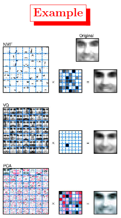
Figure:1 Non-negative matrix factorization (NMF) learns a parts-based representation of faces, whereas vector quantization (VQ) and principal components analysis (PCA) learn holistic representations.
The three learning methods were applied to a database of $m= 2,429$ facial images, each consisting of $n= 19×19$ pixels, and constituting an $n×m$ matrix $V$. All three find approximate factorizations of the form $X=WH$, but with three different types of constraints on $W$ and $H$, as described more fully in the main text and methods. As shown in the $7×7$ montages, each method has learned a set of $r= 49$ basis images.
Positive values are illustrated with black pixels ![]() and negative values with red pixels
and negative values with red pixels ![]() . A particular instance of a face :hurtrealbad: , shown at top right, is approximately represented by a linear superposition of basis images. The coefficients of the linear superposition are shown next to each montage, in a $7×7$ grid, and the resulting superpositions are shown on the other side of the equality sign. Unlike VQ and PCA, NMF learns to represent faces with a set of basis images resembling parts of faces.
. A particular instance of a face :hurtrealbad: , shown at top right, is approximately represented by a linear superposition of basis images. The coefficients of the linear superposition are shown next to each montage, in a $7×7$ grid, and the resulting superpositions are shown on the other side of the equality sign. Unlike VQ and PCA, NMF learns to represent faces with a set of basis images resembling parts of faces.
![]() Reference:
Reference:
PCA and SVD
*In case the above link is broken, click here
*In case the above link is broken, click here
Follow lecture 6 of Prof.Mitesh_IITM
- Eigenvectors can only be found for Square matrix. But, not every square matrix has eigen vectors.
- All eigen vectors are perpendicular, i.e orthogonal.
- orthonormal vectors are orthogonal and they have unit length.
- If $V$ is an orthonormal matrix then, $V^TV=I$ i.e. $V^T=V^{-1}$
PCA
- PCA decomposes a real, symmetric matrix $A$ into
eigenvectorsandeigenvalues. - Every real, symmetric matrix $A$ can be decomposed into the following expression: $A=VSV^T$.
- $V$ is an orthogonal matrix.
- $S$ is a
diagonal matrixwith all the eigen values.
- Though, any real symmetric matrix is guaranteed to have an eigen decomposition, the decomposition may not be unique.
- If a matrix is not square, then it’s eigen decomposition is not defined.
- A matrix is
singularif and only if, any of the eigenvalue is zero. - Consider A as real, symmetric matrix and $\lambda_i$ are the eigen values.
- if all $\lambda_i \gt 0$, then $\mathbf{A}$ is called positive definite matrix.
- if all $\lambda_i \ge 0$, then $\mathbf{A}$ is called positive semidefinite definite (PSD) matrix.
- PSD matricies are interesting because the gurantee that
for all x, $x^TAx \ge 0$. - PSD additionally guarantee that if $x^TAx=0$ then $x=0$.
![]() Reference:
Reference:
SVD
A is a matrix that can be seen as a linear transformation. This transformation can be decomposed in three sub-transformations: 1. rotation, 2. re-scaling, 3. rotation. These three steps correspond to the three matrices U, D, and V.
- Every matrix can be seen as a linear transformation
The transformation associated with diagonal matrices imply only a rescaling of each coordinate without rotation
- The SVD can be seen as the decomposition of one complex transformation in 3 simpler transformations (a rotation, a scaling and another rotation).
- SVD is more generic.
- SVD provides another way for factorizing a matrix, into
singular valuesandsingular vectors.- singular values::eigen values = singular vectors::eigen vectors
- Every real matrix has SVD but same is not true for PCA.
-
If a matrix is not square then PCA not applicable.
- During PCA we write $A=VSV^T$.
- However, for SVD we write $A=UDV^T$,
- where A is
m x n, U ism x m, D ism x nand V isn x n[U and V both square !!]. - U, V orthogonal matricies.
- D is diagonal matrix and not necessarily a square
-
diag(D)are thesingular valuesof the matrix A - Columns of
U(V) areleft (right) singular vectors.
- where A is
![]() Reference:
Reference:
Relation between SVD and PCA
The matrices $\mathbf{U}$, $\mathbf{D}$ and $\mathbf{V}$ can be found by transforming $\mathbf{A}$ in a
square matrixand by computing theeigenvectorsof this square matrix. The square matrix can be obtain by multiplying the matrix A by its transpose in one way or the other.
- The
left singular vectorsi.e. $\mathbf{U}$ are the eigen vectors of $\mathbf{A}\mathbf{A}^T$. Similarly, theright singular vectorsi.e. $\mathbf{V}$ are the eigen vectors of $\mathbf{A}^T\mathbf{A}$. Note that $\mathbf{A}$ might not be a square matrix but $\mathbf{A}\mathbf{A}^T$ or $\mathbf{A}^T\mathbf{A}$ are both square.- $\mathbf{A}^T\mathbf{A} = \mathbf{V}\mathbf{D}\mathbf{V}^T$ and $\mathbf{A}\mathbf{A}^T = \mathbf{U}\mathbf{D}\mathbf{U}^T$
- $\mathbf{D}$ corresponds to the eigenvalues $\mathbf{A}^T\mathbf{A}$ or $\mathbf{A}\mathbf{A}^T$ which are the same.
![]() Reference:
Reference:
How to prepare data for PCA/SVD analysis?
Before applying PCA/SVD preprocess with 3 principles:
![]() Fix count and heavy tail distribution
Fix count and heavy tail distribution
-
Sqrtany features that arecounts.logany feature with a heavy tail.
Count data and data with heavy tails can mess up the PCA.
- PCA prefers things that are
homoscedastic -
sqrtandlogare variance stabilizing transformations. It typically fixes it!
![]() Localization
Localization
If you make a histogram of a component (or loading) vector and it has really big outliers, that is localization. It’s bad. It means the vector is noise.
- Localization is noise. Regularize when you normalize.
- To address localization, I would suggest normalizing by regularized
row/column sum
Let $A$ be your matrix, define $rs$ to contain the row sums, and $cs$ to contain the column sums. define
- $D_r = Diag(\frac{1}{\sqrt{(rs + \bar{rs})}})$
- $D_c = Diag(\frac{1}{\sqrt{(cs + \bar{cs})}})$
where $\bar{rs}$ is mean(rs)
Do SVD on $D_r$ $A$ $D_c$
The use of mean(rs) is what makes it regularized.
Why it works like magic?
-
NIPS 2018- Understanding Regularized Spectral Clustering viaGraph Conductance
- Twitter thread on above paper summary
- Youtube Video on the above paper
![]() The Cheshire cat rule
The Cheshire cat rule
# One day Alice came to a fork in the road and saw a Cheshire cat in a tree.
me: "Which road do I take?"
cat: "Where do you want to go?"
me: "I don’t know"
cat: "Then, it doesn’t matter."
In unsupervised learning, we often don’t quite know where we are going.
So, is it ok to down-weight, discard, or interact the features? Try it out and see where it takes you!
![]() Reference:
Reference:
BONUS: Apply SVD on Images:
Explain PCA? Tell me the mathematical steps to implement PCA?
- In PCA, we are interested to find the directions (components) that maximize the variance in our dataset.
- PCA can be seen as:
- Learning the projection direction that captures
maximum variancein data. - Learning the projection direction that results in
smallest reconstruction error - Changing the basis in which the data is represented and transforming the features such that new features become
de-correlated(Orthogonal Principal Component)
- Learning the projection direction that captures
- Let’s assume that our goal is to reduce the dimensions of a d-dimensional dataset by projecting it onto a
k-dimensional subspace (wherek<d). So, how do we know what size we should choose fork, and how do we know if we have a feature space that represents our data well?- We will compute
eigenvectors(the components) from our data set and collect them in a so-called scatter-matrix (or alternatively calculate them from the covariance matrix). - Each of those eigenvectors is associated with an eigenvalue, which tell us about the
lengthormagnitudeof the eigenvectors. - If we observe that all the eigenvalues are of very similar magnitude, this is a good indicator that our data is already in a
goodsubspace. - If some of the eigenvalues are much much higher than others, we might be interested in keeping only those eigenvectors with the much larger eigenvalues, since they contain more information about our data distribution. Vice versa, eigenvalues that are close to 0 are less informative and we might consider in dropping those when we construct the new feature subspace.
- We will compute
-
kthEigenvector determines thekthdirection that maximizes the variance in that direction. - the corresponding
kthEigenvalue determines the variance alongkthEigenvector
![]() Tl;DR: Steps
Tl;DR: Steps
- Let $X$ is the original dataset ($n$ x $d$) [$n$: data points, $d$: dimension]
- Centered the data w.r.t mean and get the centered data: $M$ [dim: $n$ x $d$]
- Compute covariance matrix: $C=(MM^T)/(n-1)$ [dim: $d$ x $d$]
- Diagonalize it i.e do
eigen decomposition: $C = VDV^T$. $V$ is anorthogonalmatrix so $V^T = V^{-1}$ [proof]- $V$: [dim: $d$ x $k$]
- $D$: [dim: $k$ x $k$]
- Compute
principal component: $P = V\sqrt{D}$. Or you can also take the first $k$ leadingeigen vectorsfrom $V$ and the correspondingeigen valuesfrom $D$ and calculate $P$. [$P$ dim: $d$ x $k$] - Combining all:
- Apply principle component matrix $P$ on the centered data $M$ to get the transformed data projected on the principle component and thus doing
dimensionality reduction: $M^* = M P$, [$M^*$: new dataset after the PCA, dim: $n$ x $k$]. $k \lt d$, i.e.dimension reducedusingPCA.
![]() Resource:
Resource:
- pca
- a-one-stop-shop-for-principal-component-analysis
- rstudio-pubs-static
- PPT: Prof. Piyush Rai IIT Kanpur
What is disadvantage of using PCA?
- One disadvantage of PCA lies in interpreting the results of dimension reduction analysis. This challenge will become particularly telling when the data needs to be normalized.
- PCA assumes approximate normality of the input space distribution. link
- For more reading link
Why PCA needs normalization?
![]() Mitigate the effects of scale: For example, if one of the attributes is orders of magnitude higher than others, PCA tends to ascribe the highest amount of variance to this attribute and thus skews the results of the analysis. By normalizing, we can get rid of this effect. However normalizing results in spreading the influence across many more principal components. In others words, more PCs are required to explain the same amount of variance in data. The interpretation of analysis gets muddied.
Mitigate the effects of scale: For example, if one of the attributes is orders of magnitude higher than others, PCA tends to ascribe the highest amount of variance to this attribute and thus skews the results of the analysis. By normalizing, we can get rid of this effect. However normalizing results in spreading the influence across many more principal components. In others words, more PCs are required to explain the same amount of variance in data. The interpretation of analysis gets muddied.
Determinant
*In case the above link is broken, click here
*In case the above link is broken, click here
The determinant of a matrix A is a number corresponding to the multiplicative change you get when you transform your space with this matrix.
- A negative determinant means that there is a change in orientation (and not just a rescaling and/or a rotation).
![]() Reference:
Reference:
Recommendation System:
Content based recommendation:
*In case the above link is broken, click here
Using Feature vector and regression based analysis
Here the assumption is that for each of the item you have the corresponding features available.
![]() Story: Below are a table, of movie-user rating. 5 users and 4 movies. And the ratings are also provided (1-5) for some of them. We want to predict the rating for all the
Story: Below are a table, of movie-user rating. 5 users and 4 movies. And the ratings are also provided (1-5) for some of them. We want to predict the rating for all the ? unknown. It means that user $u_j$ has not seen that movie $m_i$ and if we can predict the rating for cell (i,j) then it will help us to decide whether or not to recommend the movie to the user $u_j$. For example, cell (3,4) is unknown. If by some algorithm, we can predict the rating for that cell, say the predicted rating is 4, it means if the user would have seen this movie, then he would have rated the movie 4. So we must definitely recommend this movie to the user.
| u1 | u2 | u3 | u4 | u5 | |
|---|---|---|---|---|---|
| m1 | 4 | 5 | ? | 1 | 2 |
| m2 | ? | 4 | 5 | 0 | ? |
| m3 | 0 | ? | 1 | ? | 5 |
| m4 | 1 | 0 | 2 | 5 | ? |
For content based movie recommendation it’s assumed that the features available for the content. For example if we see closely, then we can see the following patterns in the table. The bold ratings have segmented the table into 4 sub parts based on rating clustering.
| u1 | u2 | u3 | u4 | u5 | |
|---|---|---|---|---|---|
| m1 | 4 | 5 | ? | 1 | 2 |
| m2 | ? | 4 | 5 | 0 | ? |
| m3 | 0 | ? | 1 | ? | 5 |
| m4 | 1 | 0 | 2 | 5 | ? |
as if movie $m_1$, $m_2$ belong to type 1 (say romance) and $m_3$, and $m_4$ belong to type 2 (say action) and there is a clear discrimination is the rating as well.
Now for content based recommendation this types are available and then the datasets actually looks as follows
| u1 | u2 | u3 | u4 | u5 | T1 | T2 | |
|---|---|---|---|---|---|---|---|
| m1 | 4 | 5 | ? | 1 | 2 | 0.9 | 0.1 |
| m2 | ? | 4 | 5 | 0 | ? | 0.8 | 0.2 |
| m3 | 0 | ? | 1 | ? | 5 | 0.2 | 0.8 |
| m4 | 1 | 0 | 2 | 5 | ? | 0.1 | 0.9 |
where $T_1$ and $T_2$ columns are already known. Then for each of the user we can learn a regression problem with the known rating as the target vector $u_j$ and $A = [T_1,T_2]$ is the feature matrix and we need to learn the $\theta_j$ for user $j$ such that $A \theta_j = u_j$. Create the loss function and solve the optimization problem.
![]() Reference:
Reference:
Colaborative Filtering
*In case the above link is broken, click here
*In case the above link is broken, click here
![]() Story: Unlike the
Story: Unlike the content based recommendation, where the feature columns ($T_1$, $T_2$) were already given, here the features are not present. Rather they are being learnt by the algorithm. Here we assume $\theta_j$ is given i.e we know the users liking for $T_1$ and $T_2$ movies and almost similarly we formulate the regression problem but now we try to estimate the feature columns $T_k$. Then using the learnt feature we estimate the unknown ratings and then recommend those movies. Here knowing $\theta_j$
means that each user has given information regarding his/her preferences based on subset of movies and thus all the users are helping in colaborative way to learn the features.
![]() Naive Algorithm:
Naive Algorithm:
- Given $\theta_j$, learn features $T_k$. [loss function $J(T_k)$]
- Given $T_k$, learn $\theta_j$. [loss function $J(\theta_j)$]
and start with a random initialization of $\theta$ and then move back and forth between step 1 and 2.
![]() Better Algorithm:
Better Algorithm:
- combine step 1 and 2 into a single loss function $J(\theta_j,T_k)$ and solve that.
User User Colaborative Filtering
- Fix a similarity function (Jaccard similarity, cosine similarity) for two vectors. and then pick any two users profile (their rating for different movies) and calculate the similarity function which helps you to cluster the users.
-
Jaccard similaritydoesn’t consider the rating -
Cosine similarityconsider the unknown entries as 0, which causes problem as rating range is (0-5). -
Centeredcosine similarity (pearson correlation): subtract $\mu_{user}^{rating}$ from $rating_{user}$.- Missing ratings are treated as average
-
Item Item Colaborative Filtering
Almost similar to User User CF.
![]() Pros:
Pros:
- Works for any kind of item
- No need data for other user
- It’s personalized recommendation as for each user a regression problem is learnt.
- No first-rater problem, i.e. we can recommend an item to the user, as soon as it’s available in the market.
![]() Cons:
Cons:
- Finding the correct feature is hard
- Cold start problem for new user
- Sparsity
- Popularity bias
![]() Reference:
Reference:
Colaborative Filtering - Low Rank Matrix Factorization (SVD)
Evaluation of Recommending System
RMSE: Root Mean Square Error. However it doesn’t distinguish between high rating and low rating.
- Alternative: Precision $@k$ i.e. get the precision for top k items.
Deep Learning based Recommendation System
*In case the above link is broken, click here
*In case the above link is broken, click here
- For more on Recommendation System, click here.

Solve Linear Programming
min $c^Tx$ subject to: $Ax = b$, $x ≥ 0$.
The linear programming problem is usually solved through the use of one of two algorithms: either simplex, or an algorithm in the family of interior point methods.
In this article two representative members of the family of interior point methods are
introduced and studied. We discuss the design of these interior point methods on a high
level, and compare them to both the simplex algorithm and the original algorithms in
nonlinear constrained optimization which led to their genesis.
![]() [survey paper]
[survey paper]
Simplex Method
Let $A, b, c$ be an instance of the LPP, defining a convex polytope in $R^n$. Then there exists an optimal solution to this program at one of the vertices of the polytope
.
The simplex algorithm works roughly as follows. We begin with a feasible point at one of the vertices of the polytope. Then we “walk” along the edges of the polytope from vertex to vertex, in such a way that the value of the objective function monotonically decreases at each step. When we reach a point in which the objective value can decrease no more, we are finished.
![]() Reference:
Reference:
Interior Point Method
Our above question about the complexity of the LPP was answered by Khachiyan in 1979. He demonstrated a worst-case polynomial time algorithm for linear programming dubbed the ellipsoid method [Kha79] in which the algorithm moved across the interior of the feasible region, and not along the boundary like simplex. Unfortunately the worst case running time for the ellipsoid method was high: $O(n^6L^2)$, where n is the number of variables in the problem and L is the number of the bits in the input. Moreover, this method tended to approach the worst-case complexity on nearly all inputs, and so the simplex algorithm remained dominant in practice. This algorithm was only partially satisfying to researchers: was there a worst-case polynomial time algorithm for linear programming which had a performance that rivalled the performance of simplex on day-to-day problems? This question was answered by Karmarkar in 1984. He produced a polynomial-time algorithm — soon called the projective algorithm — for linear programming that ran in much better time: $O(n^{3.5}L^2)$ [Kar84].
![]() Reference:
Reference:
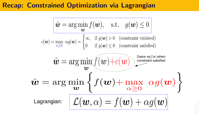
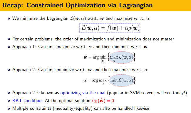
First Order Method - The KKT Conditions and Duality Theory
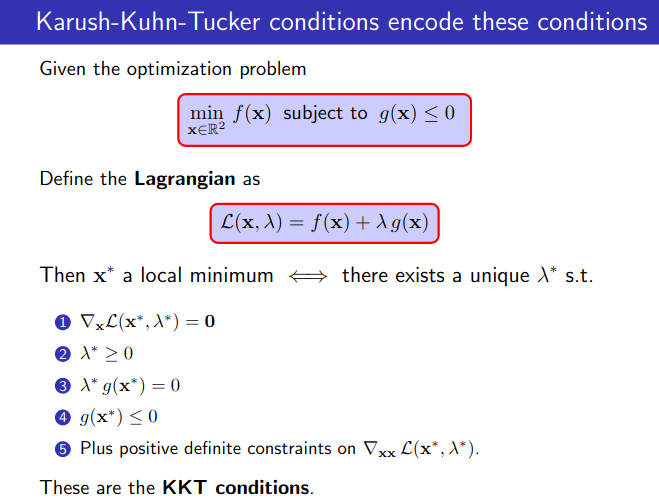
![]() KKT Conditions:
KKT Conditions:
- Stationarity $\nabla_x L(x,\lambda,\mu)=0$
- Primal feasibility, $g(x) \leq 0$ (for minimization problem)
- Dual feasibility, $\lambda \geq 0, \mu \geq 0$
- Complementary slackness, $\lambda g(x) = 0$ and $\mu h(x)=0$
![]() Resource
Resource
What is LBFGS algorithm?
- In numerical optimization, the
Broyden–Fletcher–Goldfarb–Shanno(BFGS) algorithm is aniterative methodfor solvingunconstrained nonlinear optimizationproblems. - The BFGS method belongs to quasi-Newton methods, a class of hill-climbing optimization techniques that seek a stationary point of a (preferably twice continuously differentiable) function. For such problems, a necessary condition for optimality is that the gradient be zero. Newton’s method and the BFGS methods are not guaranteed to converge unless the function has a quadratic Taylor expansion near an optimum. However, BFGS can have acceptable performance even for non-smooth optimization instances.
![]() Resource:
Resource:
Second-Order Methods: Newton’s Method
- GD and variants only use first-order information (the gradient)
-
 Second-order information often tells us a lot more about the function’s
 shape,curvature, etc.- Newton’s method is one such method that uses second-order information.
- At each point, approximate the function by its quadratic approx. and minimize it
- Doesn’t rely on gradient to choose $w_{(t+1)}$Instead, each step directly jumps to the minima of quadratic approximation.
- No learning rate required

- Very fast if $f(w)$ is convex. But expensive due to Hessian computation/inversion.
- Many ways to approximate the Hessian (e.g., using previous gradients); also look at
L-BFGS
Second order Derivative
- In calculus, the second derivative, or the second order derivative, of a function $f$ is the derivative of the derivative of $f$. Roughly speaking, the second derivative measures how the
rate of change of a quantityis itselfchanging;- For example, the second derivative of the position of a vehicle with respect to time is the instantaneous acceleration of the vehicle, or the rate at which the velocity of the vehicle is changing with respect to time.
![]() On the
On the graph of a function, the second derivative corresponds to the curvature or concavity of the graph.
- The graph of a function with a
positive second derivativeisupwardly concave, - The graph of a function with a
negative second derivativecurves in the opposite way.

A plot of $f( x ) = sin ( 2 x )$ from $-\pi/4$ to $5\pi/4$ . The tangent line is blue where the curve is
concave up, green where the curve isconcave down, and red at the inflection points (0, $\pi/2$, and $\pi$).
![]() Reference:
Reference:
Gradient, Jacobian, Hessian, Laplacian and all that
![]() Gradient: To generalize the notion of derivative to the multivariate functions we use the gradient operator.
Gradient: To generalize the notion of derivative to the multivariate functions we use the gradient operator.
Gradient vector gives us the magnitude and direction of maximum change of a multivariate function.
![]() Jacobian: The Jacobian operator is a generalization of the derivative operator to the vector-valued functions. As we have seen earlier, a vector-valued function is a mapping from $f:ℝ^n \rightarrow ℝ^m$ hence, now instead of having a scalar value of the function $f$, we will have a mapping $[x_1,x_2, \dots ,x_n] \rightarrow [f_1,f_2, \rightarrow,f_n]$. Thus, we now need the rate of change of each component of $f_i$ with respect to each component of the input variable $x_j$, this is exactly what is captured by a matrix called Jacobian matrix $J$:
Jacobian: The Jacobian operator is a generalization of the derivative operator to the vector-valued functions. As we have seen earlier, a vector-valued function is a mapping from $f:ℝ^n \rightarrow ℝ^m$ hence, now instead of having a scalar value of the function $f$, we will have a mapping $[x_1,x_2, \dots ,x_n] \rightarrow [f_1,f_2, \rightarrow,f_n]$. Thus, we now need the rate of change of each component of $f_i$ with respect to each component of the input variable $x_j$, this is exactly what is captured by a matrix called Jacobian matrix $J$:
![]() Hessian: The gradient is the first order derivative of a multivariate function. To find the second order derivative of a multivariate function, we define a matrix called a Hessian matrix. It describes the
Hessian: The gradient is the first order derivative of a multivariate function. To find the second order derivative of a multivariate function, we define a matrix called a Hessian matrix. It describes the local curvature of a function of many variables.
Suppose $f : ℝ^n \rightarrow ℝ$ is a function taking as input a vector $x ∈ ℝ^n$ and outputting a scalar $f(x) ∈ ℝ$. If all second partial derivatives of $f$ exist and are continuous over the domain of the function, then the Hessian matrix $H$ of f is a square $n \times n$ matrix, usually defined and arranged as follows
$ H = \begin{vmatrix} \frac{\delta^2 f}{\delta x_1^2} , \frac{\delta^2 f}{\delta x_1 x_2}\\ \frac{\delta^2 f}{\delta x_2 x_1} , \frac{\delta^2 f}{\delta^2 x_2}\\ \end{vmatrix} $
The Hessian matrix of a function f is the Jacobian matrix of the gradient of the function f ; that is: $H(f(x)) = J(\nabla f(x))$.
![]() Laplacian: The trace of the Hessian matrix is known as the Laplacian operator denoted by $\nabla^2$
Laplacian: The trace of the Hessian matrix is known as the Laplacian operator denoted by $\nabla^2$
Reference:
Why does L1 regularization induce sparse models?
*In case the above link is broken, click here
*In case the above link is broken, click here
Clustering Algorithm
- When data set is very large, can’t fit into memory, then K means algorithm is not a good algorithm. Rather use Bradley-Fayyad-Reina (BFR) algorithm.
BFR (Bradley, Fayyad and Reina)
The BFR algorithm, named after its inventors Bradley, Fayyad and Reina, is a variant of k-means algorithm that is designed to cluster data in a high-dimensional Euclidean space. It makes a very strong assumption about the shape of clusters:
- They must be normally distributed about a centroid
 .
. - The mean and standard deviation for a cluster may differ for different dimensions, but the dimensions must be independent.
![]() Strong Assumption:
Strong Assumption:
- Each cluster is
normally distributedaround a centroid in Euclidean space - Normal distribution assumption implies that clusters looks like
axis-aligned ellipses, i.e. standard deviation is maximum along one axis and minimum w.r.t other.
![]() Reference:
Reference:
How to implement regularization in decision tree, random forest?
In Narrow sense, Regularization (commonly defined as adding Ridge or Lasso Penalty) is difficult to implement for Trees.
- Tree is a heuristic algorithm.
In broader sense, Regularization (as any means to prevent overfit) for Trees is done by:
- Limit max. depth of trees
- Ensembles / bag more than just 1 tree
- Set stricter stopping criterion on when to split a node further (e.g. min gain, number of samples etc.)
![]() Resource:
Resource:
Why random column selection helps random forest?
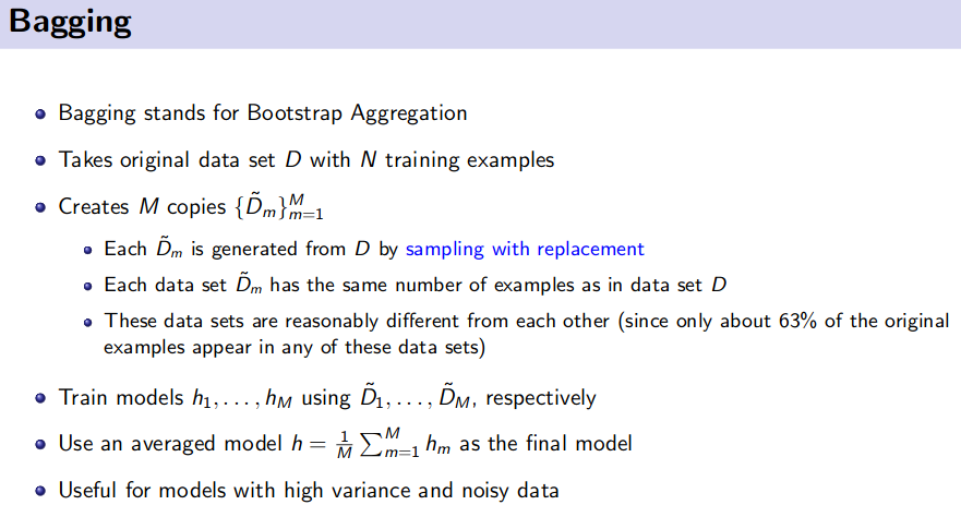
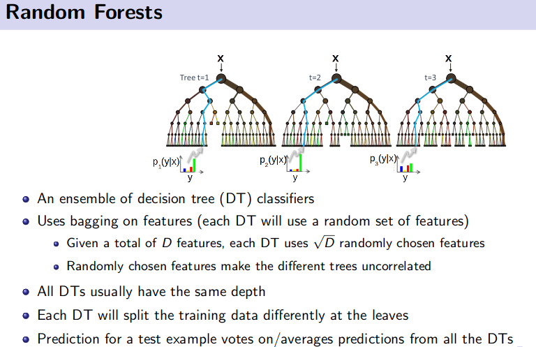
Random forest algorithm comes under the Bootstrap Algorithm a.k.a Bagging category whose primary objective is to reduce the variance of an estimate by averaging many estimates.
-
 Sample datasets without replacement
- In bootstarp algorithm
Mdecision trees are trained onMdatasets which are sampledwithout replacementfrom the original datasets. Hence each of the sampled data will have duplicate data as well as some missing data, which are present in the original data, as all the sampled datasets have same length. Thus, these bootstrap samples will have diversity among themselves, resulting the model to be diverse as well.
- In bootstarp algorithm
Along with the above methods Random Forest also does the following:
-
 Random subset of feature selection for building the tree
- This is known as subspace sampling
- Increases the diversity in the ensemble method even more
- Tree training time reduces.
-
 IMPORTANT: Also simply running the same model on different sampled data will produce highly correlated predictors, which limits the amount of variance reduction that is possible. So RF tries to decorrelate the base learners by learning trees based on a randomly chosen subset of input variables, as well as, randomly chosen subset of data cases.
![]() Reference:
Reference:
- source: 1. Kevin Murphy, 2. Peter Flach
- ref
Overfitting in Random Forest
-
To avoid over-fitting in random forest, the main thing you need to do is optimize a tuning parameter that governs the number of features that are randomly chosen to grow each tree from the bootstrapped data. Typically, you do this via k-fold cross-validation, where k∈{5,10}, and choose the tuning parameter that minimizes test sample prediction error. In addition, growing a larger forest will improve predictive accuracy, although there are usually diminishing returns once you get up to several hundreds of trees.
-
For decision trees there are two ways of handling overfitting: (a) don’t grow the trees to their entirety (b) prune. The same applies to a forest of trees - don’t grow them too much and prune.
![]() Reference:
Reference:
- SO:random-forest-tuning-tree-depth-and-number-of-trees
- statsexchange:random-forest-how-to-handle-overfitting
How to avoid Overfitting?
Overfitting means High Variance
Steps to void overfitting:
- Cross Validation
- Train with more data
- Remove feature
- Early stopping
- Regularizations
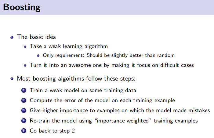
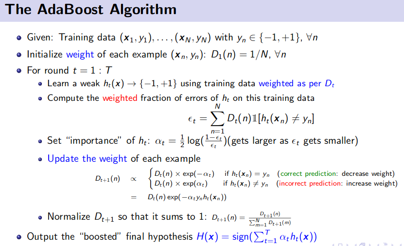
- Ensembling
How to avoid Underfitting?
- Add more features
- Add more data
- Decrease the amount of regularizations
Gaussian Processing
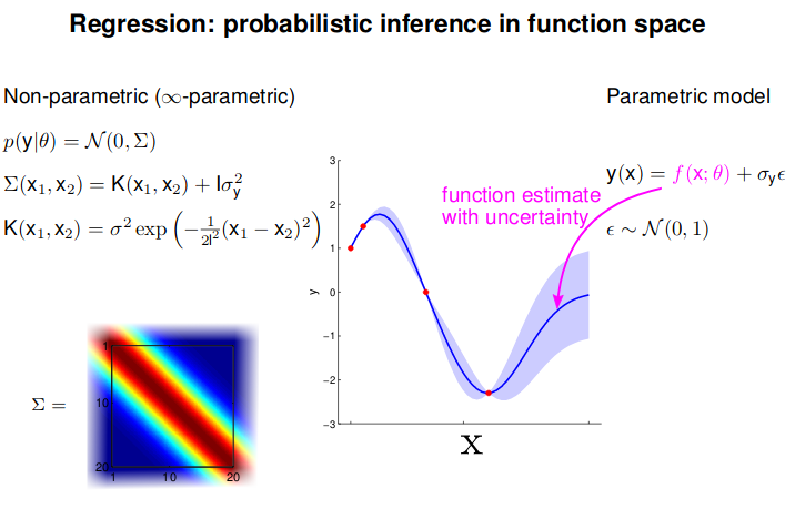
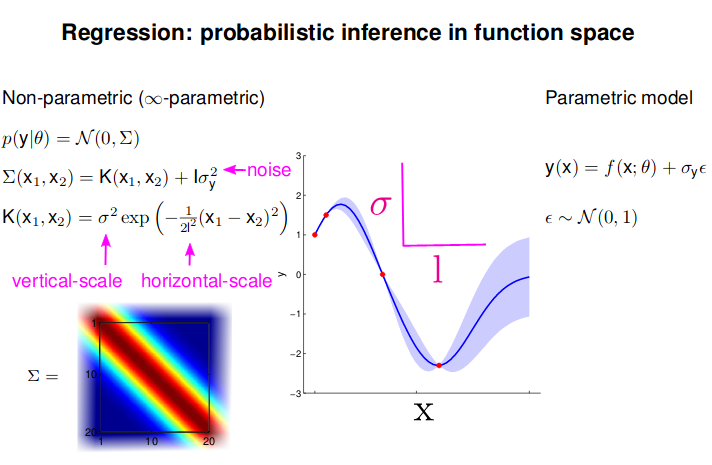

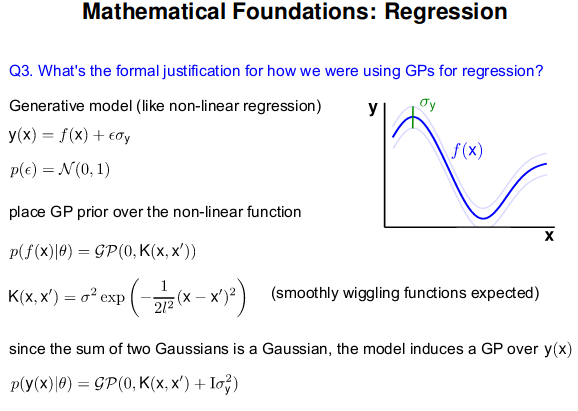
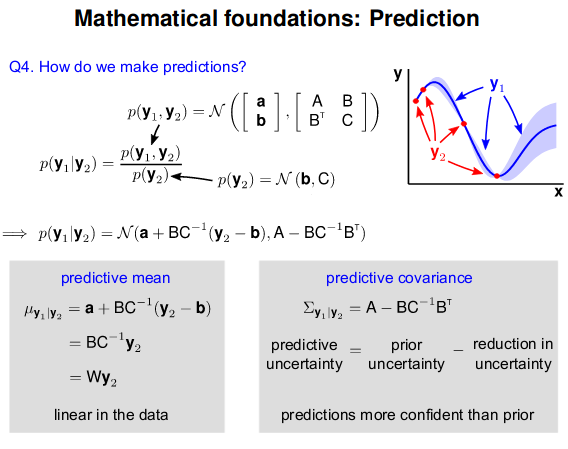
- GP: Collection of random variables, any finite number of which are Gaussian Distributed
- Easy to use: Predictions correspond to models with infinite parameters
- Problem: $N^3$ complexity
![]() Reference:
Reference:
K-Means Clustering (Unsupervised Learning)
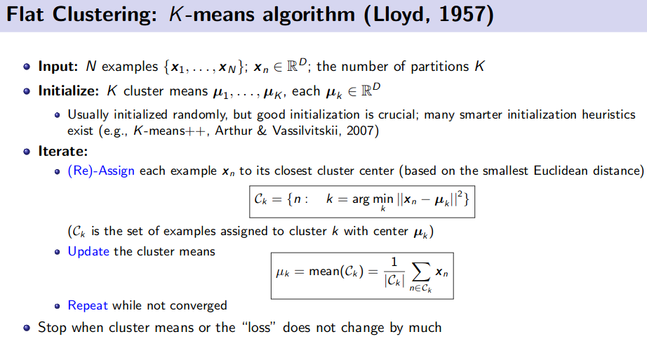
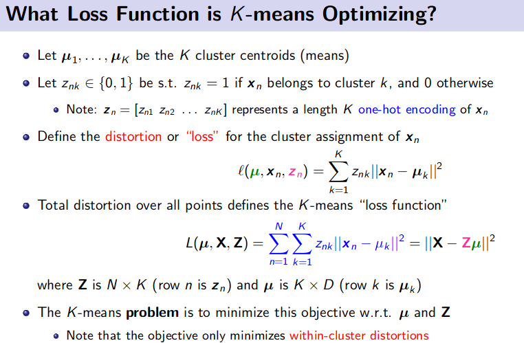
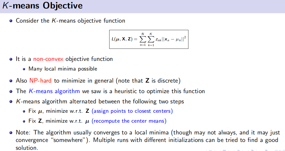
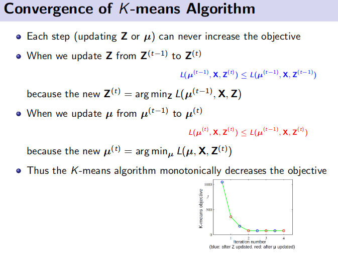
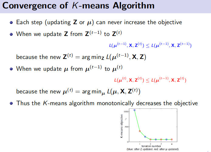
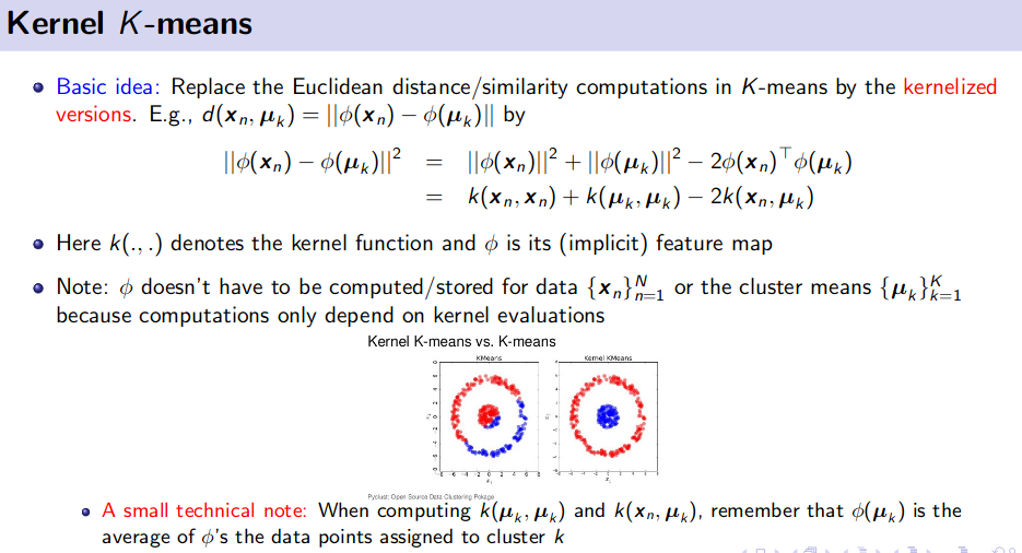
![]() Resource:
Resource:
PCA and Kernel PCA
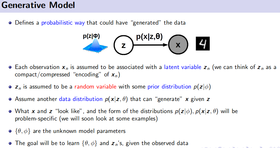
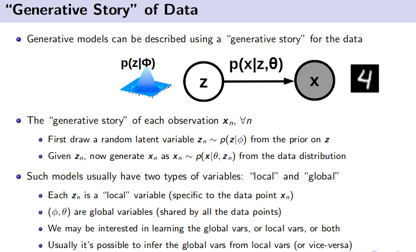
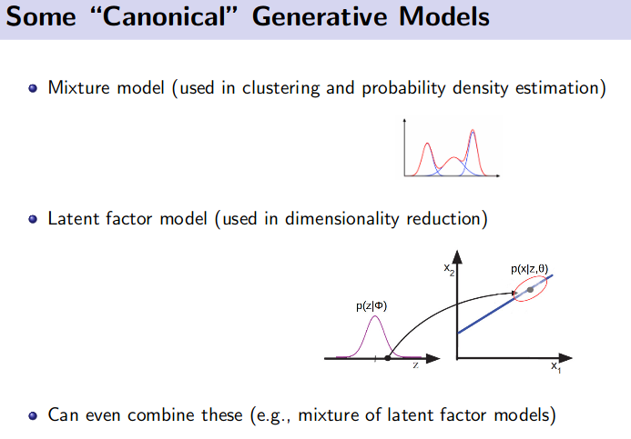
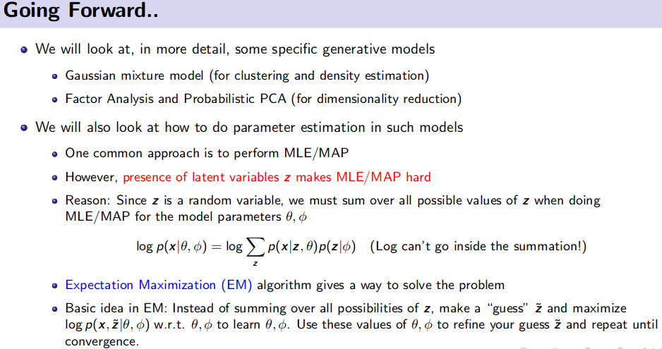
Generative Model (Unsupervised Learning)
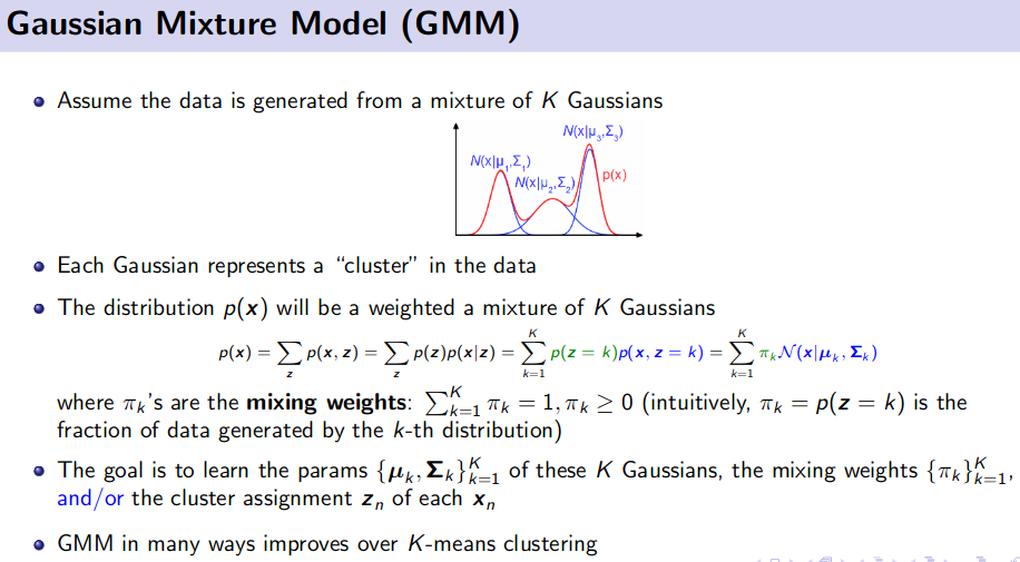
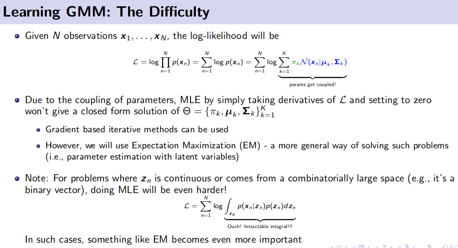
![]() Resource:
Resource:
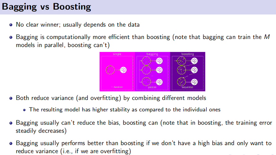
Ensemble Method (Bagging and Boosting)
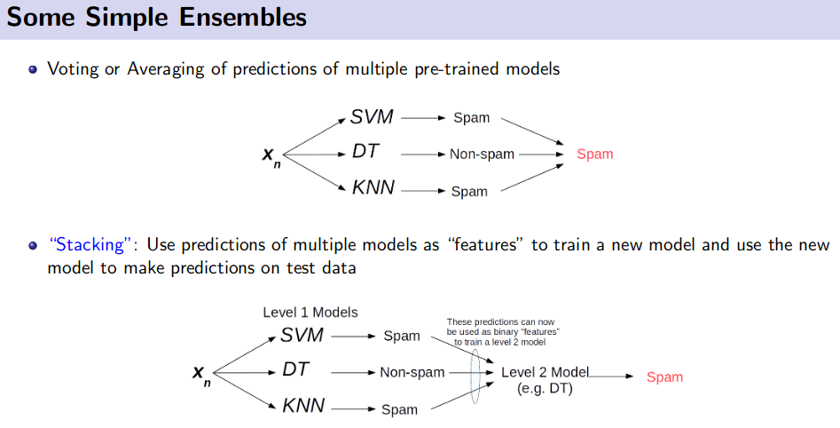
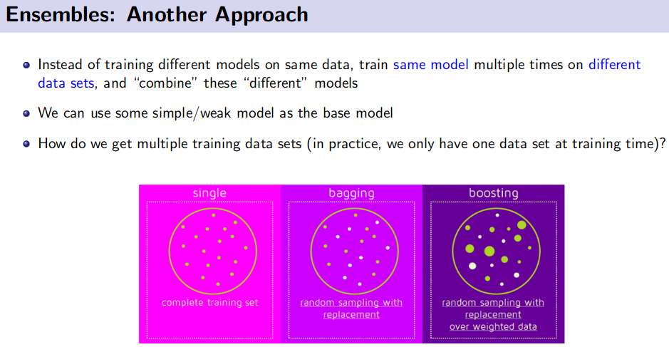
![]() Reference:
Reference:
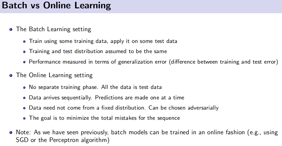
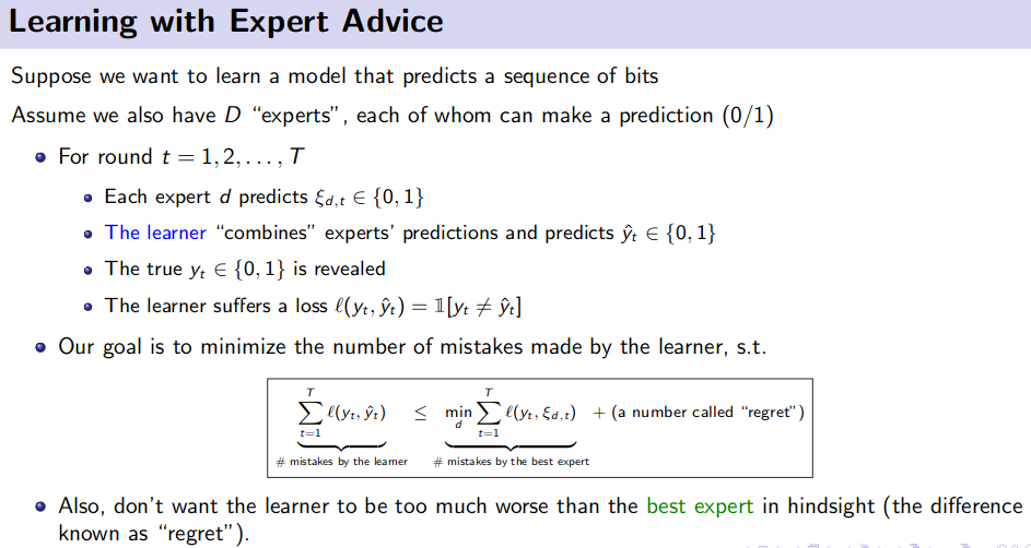
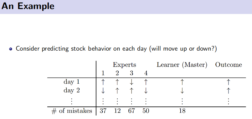
Online Learning
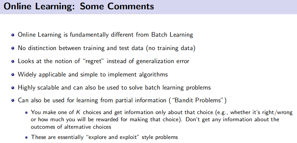
![]() Resource:
Resource:
Model/ Feature Selection and Model Debugging
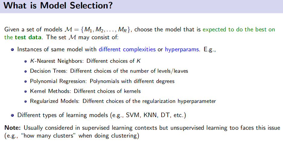
Different strategies:
- Hold-out/ Validation data
- Problem: Wastes training time
- K-Fold Cross Validation (CV)
- Leave One Out (LOO) CV
- Problem: Expensive for large $N$.
- But very efficient when used for selecting the number of neighbors to consider in nearest neighbor methods. (reason: NN methods require no training)
- Random Sub-sampling based Cross-Validation
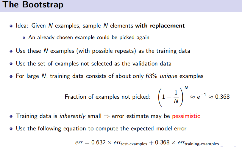
- Bootstrap Method
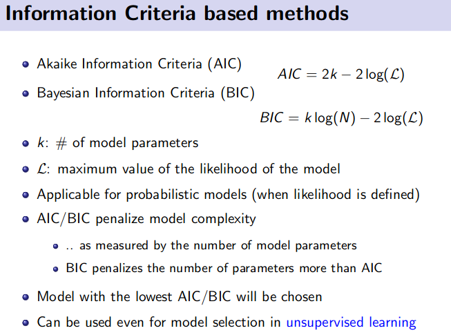
- Information Criteria based methods
Debugging Learning Algorithm

Resource:
Bayesian Machine Learning
Coursera - Bayesian Methods for Machine Learning
Finding similar sets from millions or billions data
Techniques:
- Shingling: converts documents, emails etc to set.
- Min-hashing: Convert large sets to short signature, while preserving similarity
- Locality-Sensitive-Hashing: Focus on pair of signatures likely to be similar.
![]() Reference:
Reference:
Lecture 12, 13, 14 of below playlist
 Top Pick for Interview - Depth and Breadh
- Entropy
- KL divergence
- Kolmogorov complexity
- Jacobian and Hessian
- Linear independence
- Determinant
- Eigenvalues and Eigenvectors
- PCA and SVD
- The norm of a vector
- Independent random variables
- Expectation and variance
- Central limit theorem
- Law of Large Number
- Gradient descent and SGD
- The dimension of gradient and hessian for a neural net with 1k params
- What is SVM
- Quadratic optimization
- What to do when a neural net overfits
- What is autoencoder
- How to train an RNN
- How decision trees work
- Random forest and GBM
- How to use random forest on data with 30k features
- Favorite ML algorithm - tell about it in details

